The Amazing, Globular Fibonacci Sphere

How do you place a number of points on the surface of a sphere at equidistant positions? You might first look to a geographic coordinate system using latitude and longitude, or some similar method for regularly incrementing spherical coordinates, but most of these cannot achieve the equidistant spacing we desire. The solution, however, lies somewhere between sunflowers and parabolas.

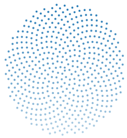
Points on a disk

In his paper, “A Better Way To Construct The Sunflower Hood”, Vogel shows that using a Fermat spiral that increments at 137.5 degrees best represents the position of disk florets at the center of the sunflower. Why 137.5 degrees? That number is, approximately, the golden angle, which is formed by the most irrational number, the golden mean. That extreme irrationality lends itself to a lack of periodicity of points on concentric spirals.

  
  import numpy as np
  import matplotlib.pyplot as plt
  import mpl_toolkits.mplot3d.axes3d as ax3d

  def fibonacci_disc(numpts: int):

      ga = np.pi * (3 - np.sqrt(5)) # golden angle
	  theta = np.arange(numpts) * ga

      radius = np.sqrt(np.arange(numpts) / float(numpts))
	  x = radius * np.cos(theta)
	  y = radius * np.sin(theta)

      # Display points in a scatter plot
	  fig = plt.figure()
	  ax = fig.add_subplot(111, projection='3d')
	  ax.scatter(x, y, [0] * numpts)
	  plt.axis('off')
	  plt.show()
  

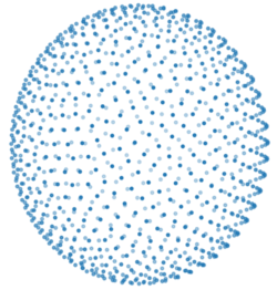
Points on a sphere

Converting from the 2D case to the 3D case is quite simple! Conceptually, you assign each of your points to a different, equidistant height along the length of the sphere’s diameter. At each height, a similarly incremented angle (again by the golden angle at each step) determines, along with the sphere’s radius at that height, determines where the point lies on the sphere’s surface. In python that looks like this:

  
  import matplotlib.pyplot as plt
  import mpl_toolkits.mplot3d.axes3d as ax3d
  import numpy as np

  def fibonacci_sphere(numpts: int):
      ga = (3 - np.sqrt(5)) * np.pi # golden angle

      # Create a list of golden angle increments along tha range of number of points
	  theta = ga * np.arange(numpts)

      # Z is a split into a range of -1 to 1 in order to create a unit circle
	  z = np.linspace(1/numpts-1, 1-1/numpts, numpts)

      # a list of the radii at each height step of the unit circle
	  radius = np.sqrt(1 - z * z)

      # Determine where xy fall on the sphere, given the azimuthal and polar angles
	  x = radius * np.cos(theta)
	  y = radius * np.sin(theta)

      # Display points in a scatter plot
	  fig = plt.figure()
	  ax = fig.add_subplot(111, projection='3d')
	  ax.scatter(x, y, z)
	  plt.axis('off')
	  plt.show()
  

Points on a spherical cap

In the many instances where you might not want to cover the entire sphere, you can generalize the above process to any height on the sphere. I do it in a non-optimal, but more easily understandable, way here. We still calculate all points on the sphere, but display only the number of points that are proportional to the desired height of the cap (versus the total sphere height).

To what end?

Before I took this golden-angled path, I wanted a way to place equdistant points on a spherical cap in order to more properly represent sensor detections for sensors with a significant field of view, and for which the max distance forms a spherical cap. Now, for most sensors, and for most systems, adding either a single point to your map would likely work fine for the purposes of rough obstacle avoidance. Given the small resolution of the voxels that form my map, and given the fine navigation I’m looking to perform in tight spaces, I opted for this fine-grained representation of the sensor detection cap. I hope you, as well, find some benefit from this exloratory endeavour!